ICP匹配原理实践

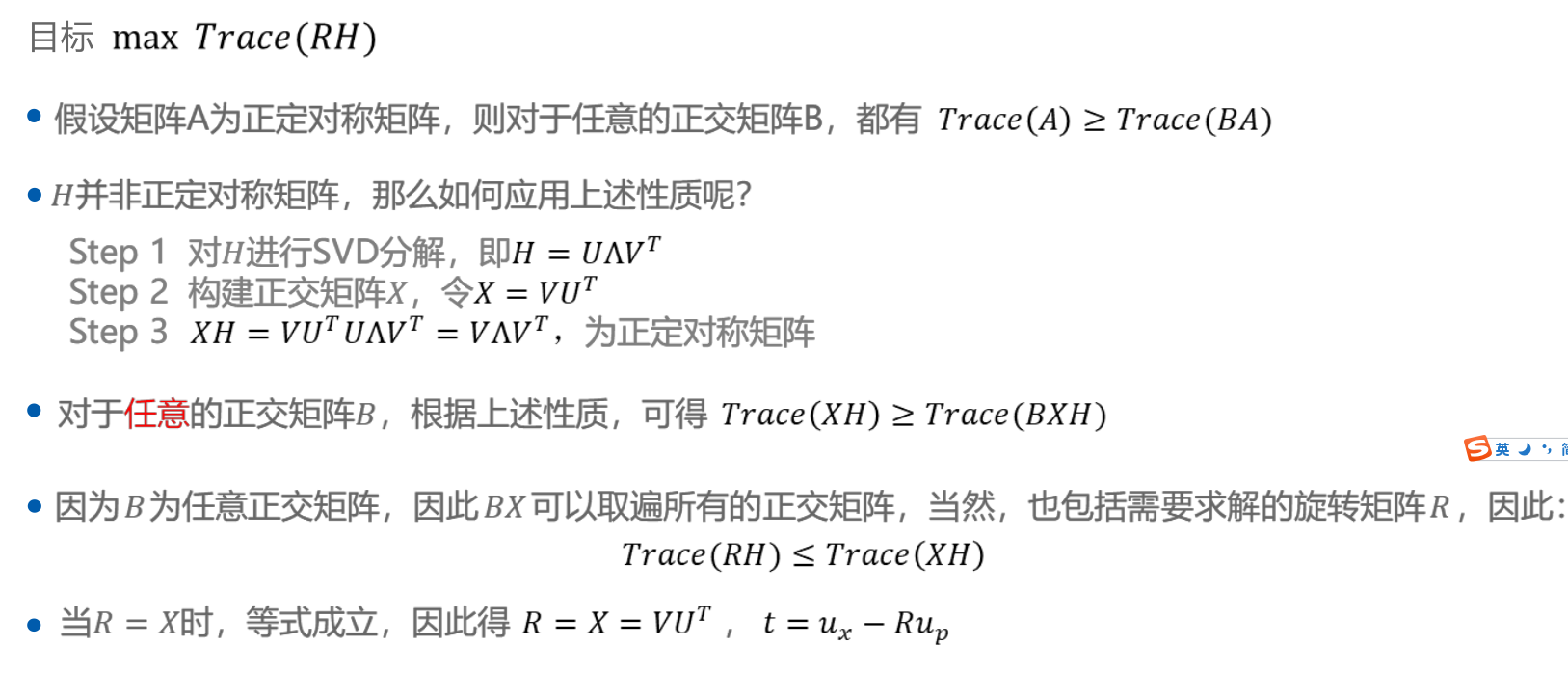
迭代最近点算法 Iterative Closest Point (ICP）可以是点云中经常用于匹配的配准算法，可以求解两组点之间的位姿关系。本文以2D激光雷达为例子，讲解如何使用ICP，并且加入ROS2的仿真中去。

data= array([[-0.32829776,  1.77534997],
       [-0.31087252,  1.79521136],
       [-0.27960942,  1.79588288],
       [-0.25491268,  1.80528362],
       [-0.22668769,  1.8092163 ],
       [-0.21100112,  1.83158204],
       [-0.19026372,  1.84654157],
       [-0.16153892,  1.84884591],
       [-0.14361304,  1.86819745],
       [-0.11789602,  1.8748071 ],
       ...
       ])

为一个shape=(n, 2)的雷达数据

雷达点的坐标转换

坐标点变换矩阵，绕着原点逆时针旋转

$$R =\begin{bmatrix} \cos\theta&-\sin\theta\\ \sin\theta&\cos\theta \end{bmatrix}$$

若有一个点$x=(x_0,y_0)$，逆时针旋转$\theta$度，则应该计算为

$$x=x_0\cos\theta-y_0\sin\theta\\ y=x_0\sin\theta+y_0\cos\theta\tag{1}$$

转换为矩阵为R@x.T即可

因此，坐标变换应该为R@data.T即可，注意结果为shape=(2,n)。

齐次坐标系变换

倘若在旋转的基础之上还需要平移$t=(t_x,t_y)$，则

$$x=x_0\cos\theta-y_0\sin\theta+t_x\\ y=x_0\sin\theta+y_0\cos\theta+t_y\tag{2}$$

写为矩阵的形式应该为

$$\begin{bmatrix} \cos\theta&-\sin\theta&t_x\\ \sin\theta&\cos\theta&t_y\\ 0&0&1 \end{bmatrix} \begin{bmatrix} x_0\\ y_0\\ 1 \end{bmatrix}\tag{3}$$

因此应该矩阵的乘法，首先需要对数据加一个列的1

data = np.hstack((data, np.ones((test_point.shape[0], 1))))

坐标变换应该为T_1@data.T，其中$T_1$为（3）左边的矩阵，注意结果为shape=(3, n)

如果需要计算多次平移和旋转

则只需要继续左乘即可T_2@T_1@data.T

已知对应点关系的ICP

def icp(y_data_pre, y_data_now):
    """
    y_data_pre: shape=(n, 2)
    y_data_now: the same snow_tmhape of y_data_pre = (n, 2)
    
    return: R and t. The transformation from pre to now
    """
    total_R = np.eye(3)
    
    pre_tm, now_tm = y_data_pre, y_data_now

    pre_t, now_t = pre_tm - np.mean(pre_tm, axis=0), now_tm - np.mean(now_tm, axis=0)

    W = np.zeros((2,2))

    for i in range(pre_t.shape[0]):
        W += pre_t[i:i+1].T @ now_t[i:i+1]

    U, sigma, V = np.linalg.svd(W)
    R = V @ U.T
    t = np.mean(now_tm, axis=0) - R@np.mean(pre_tm, axis=0).T
    
    return trans_to_isometry2d(R, t)

上面这个函数输入是两个点云，并且shape=(n, 2)

返回的是一个3x3的欧式变换矩阵

$$\begin{bmatrix} R & t\\ 0&1 \end{bmatrix} \tag{4}$$

$R$是一个二维的旋转矩阵，$t$表示的是平移向量。

下面介绍ICP的具体步骤

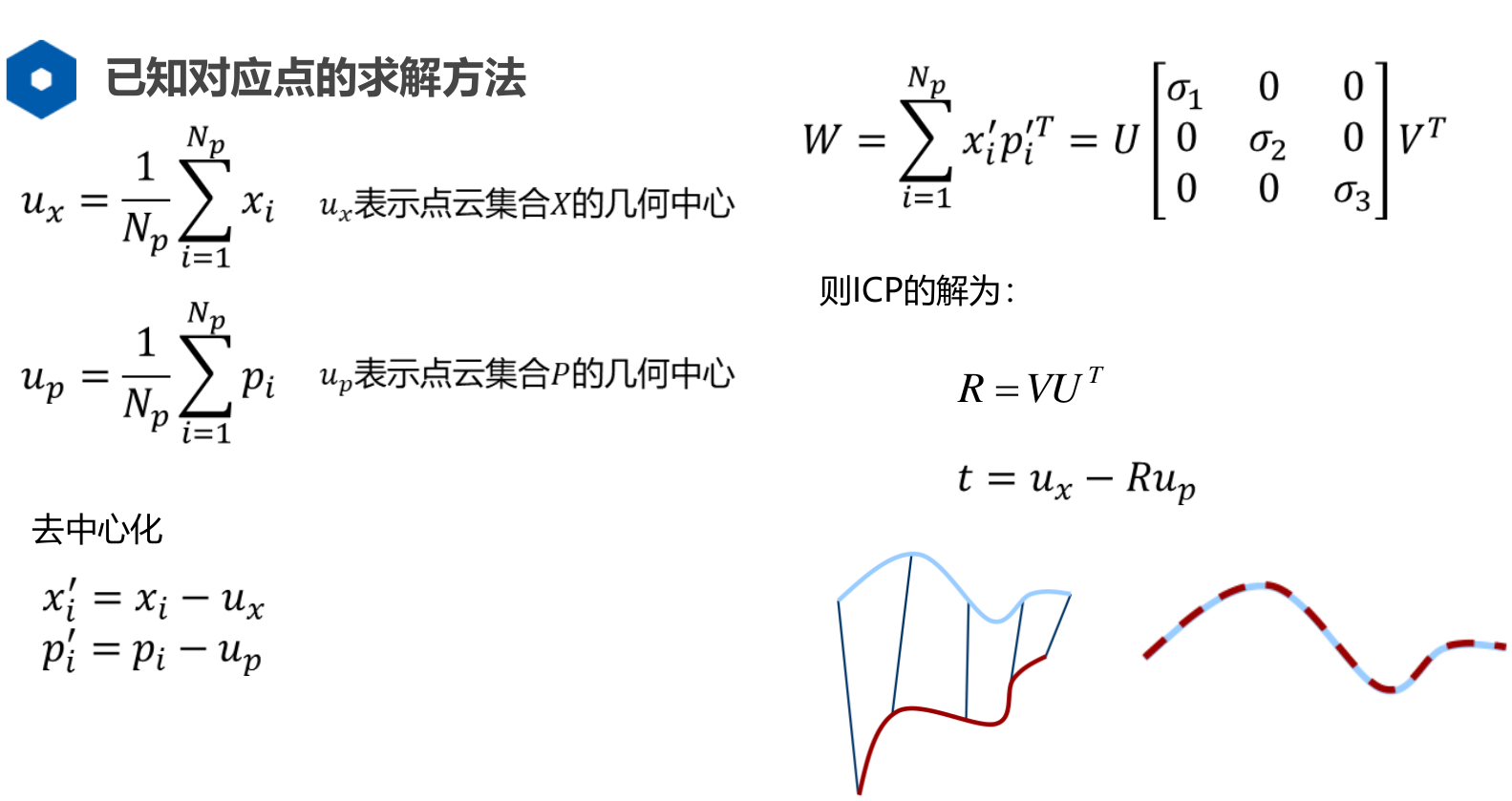
步骤一：去中心化

pre_t, now_t = pre_tm - np.mean(pre_tm, axis=0), now_tm - np.mean(now_tm, axis=0)

步骤二：计算矩阵W

$$W=\sum_{i=1}^Nx_i'p_i$$

其中，$x_i,p_i$分别代表两块点云中的点。

for i in range(pre_t.shape[0]):
    W += pre_t[i:i+1].T @ now_t[i:i+1]

步骤三：SVD分解，求解R

假设对W的SVD分解结果为

$$W=U\begin{bmatrix} \sigma_1 & 0&0\\ 0&\sigma_2&0\\ 0&0&\sigma_3 \end{bmatrix}V^T$$

则ICP的解为

$$R = VU^T$$

U, sigma, V = np.linalg.svd(W)
R = V @ U.T

步骤四：求解t

$$t=u_x-Ru_p$$

其中$u_x$和$u_p$分别表示两块点云的几何中心点

t = np.mean(now_tm, axis=0) - R@np.mean(pre_tm, axis=0).T

案例

数据生成

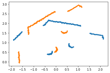
下面这段代码，我们生成了已知对应点的两个点云y_data_now以及y_data_pre

y_data_now是通过y_data_pre逆时针旋转45度，并且平移了[0.5, 0.5]得到

import matplotlib.pyplot as plt
import numpy as np

pre = np.array([2.2172601222991943, 2.222874402999878, 2.205129384994507, 2.1986029148101807, 2.1858696937561035, 2.1957268714904785, 2.1969168186187744, 2.183438539505005, 2.190436601638794, 2.1827948093414307, 2.1837754249572754, 2.2076597213745117, 2.177976131439209, 2.1731295585632324, 2.185473918914795, 2.1618497371673584, 2.1733145713806152, 2.181365728378296, 2.1715705394744873, 2.1802971363067627, 2.1772191524505615, 2.1959474086761475, 2.1840665340423584, 0.5597301125526428, 0.5485700964927673, 0.5352249145507812, 0.5243845582008362, 0.5171780586242676, 0.49347609281539917, 0.500745415687561, 0.5121733546257019, 0.5016278624534607, 0.5036090016365051, 0.5045422911643982, 0.5057468414306641, 0.48604974150657654, 0.4834277033805847, 0.49271881580352783, 0.4894062876701355, 0.47749894857406616, 0.47225064039230347, 0.47715726494789124, 0.48048126697540283, 0.4855308532714844, 0.4973067045211792, 0.4793863892555237, 0.4819462299346924, 0.4518357813358307, 0.48269888758659363, 0.4819696545600891, 0.4706280529499054, 0.4844808280467987, 0.4945412874221802, 0.5085427761077881, 0.49312782287597656, 0.500328540802002, 0.49513912200927734, 0.4999622404575348, 0.5043498277664185, 0.5245479345321655, 0.541199266910553, 0.5258843302726746, 0.5450403690338135, 0.5684719681739807, 1.9805926084518433, 1.992526888847351, 1.988566279411316, 2.026911735534668, 2.0081746578216553, 2.046605110168457, 2.0853240489959717, 2.075857162475586, 2.0827317237854004, 2.1258904933929443, 2.14408540725708, 2.169947624206543, 2.1946492195129395, 2.1616666316986084, 2.172661781311035, 2.154602289199829, 2.1330761909484863, 2.13897442817688, 2.137460470199585, 2.13767671585083, 2.098261594772339, 2.0943005084991455, 2.0957398414611816, 2.0956742763519287, 2.087766170501709, 2.091048002243042, 2.1002793312072754, 2.0828135013580322, 2.063037872314453, 2.0801477432250977, 2.062371015548706, 2.0871875286102295, 2.083261013031006, 2.0732927322387695, 2.08502197265625, 2.0588319301605225, 2.0332274436950684, 2.0723254680633545, 2.0552995204925537, 2.057854413986206, 2.069274663925171, 2.032874822616577, 2.0648837089538574, 2.072674512863159, 2.062706470489502, 2.045621633529663, 2.0590219497680664, 2.059302568435669, 2.0588607788085938, 2.0754079818725586, 2.0734634399414062, 2.0726094245910645, 2.0943069458007812, 2.0891125202178955, 2.0705318450927734, 2.0788536071777344, 2.10817289352417, 2.1069400310516357, 2.109229326248169, 2.101857900619507, 2.1055896282196045, 2.115345001220703, 2.119300127029419, 2.1327497959136963, 2.1400115489959717, 2.1617844104766846, 2.134272575378418, 2.146404266357422, 2.1694626808166504, 2.1619796752929688, 2.190279006958008, 2.1727895736694336, 1.1113004684448242, 1.100041389465332, 1.0575999021530151, 1.0355123281478882, 1.0419548749923706, 1.037386417388916, 1.0438101291656494, 0.994590163230896, 1.027056336402893, 1.0087417364120483, 1.0027227401733398, 1.0239629745483398, 1.0005853176116943, 1.017919659614563, 1.0248370170593262, 1.0239020586013794, 1.0181171894073486, 1.0272765159606934, 1.0323562622070312, 1.0463443994522095, 1.0655380487442017, 1.0990997552871704, 2.132075071334839, 2.1586179733276367, 2.149562358856201, 2.172996759414673, 2.202742576599121, 2.2174174785614014, 2.2322938442230225, 2.2515151500701904, 2.286550283432007, 2.2972664833068848, 2.330606698989868, 2.3576974868774414, 2.3825862407684326, 2.4172351360321045, 2.4361069202423096, 2.461888313293457, 2.5018298625946045, 2.4925389289855957, 2.4813530445098877, 2.452197313308716, 2.4803617000579834, 2.4636669158935547, 2.4398932456970215])

def convert_scan_to_pointcloud(scan):
    """
    把激光消息转换为激光坐标系下的二维点云
    """
    angle_min=-1.0466699600219727
    angle_max=1.0466699600219727
    angle_increment=0.011629666201770306
    n = len(scan)
    pcs = np.zeros((n, 2))
    angle = angle_min
    for i in range(n):
        if scan[i] < 0.07999999821186066 or scan[i] > 6.0:
            continue
        angle += angle_increment
        # 计算单个值的三角函数，math比numpy的快
        lx = scan[i] * math.sin(angle)
        ly = scan[i] * math.cos(angle)
        if not lx or not ly:
            continue
        pcs[i][0] = lx
        pcs[i][1] = ly

    return pcs

y_data_pre = convert_scan_to_pointcloud(pre)
# 为已知的点云进行变换，假设为旋转pi/8,平移距离为（1，1）
theta = 3.1415926/4
t = np.array([0.5, 0.5])
R = np.array([[np.cos(theta), -np.sin(theta)], [np.sin(theta), np.cos(theta)]])
y_data_now = (R @ y_data_pre.T).T + t
print("the rotation matrix should be:\n {}".format(R))

the rotation matrix should be:
 [[ 0.70710679 -0.70710677]
 [ 0.70710677  0.70710679]]

# 画出两点云
plt.scatter(y_data_pre[:,0], y_data_pre[:,1], marker='o', s=10)
plt.scatter(y_data_now[:,0], y_data_now[:,1], marker='o', s=10)

通过ICP进行相对位姿计算

icp(y_data_pre, y_data_now)

计算结果为：

array([[ 0.70710679, -0.70710677,  0.5       ],
       [ 0.70710677,  0.70710679,  0.5       ],
       [ 0.        ,  0.        ,  1.        ]])

这和我们所预期的结果完全一致。

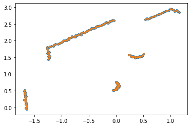
下面我们画出旋转后的结果

y_data_from_icp = (icp(y_data_pre, y_data_now) @ np.hstack((y_data_pre, np.ones((y_data_pre.shape[0], 1)))).T).T
plt.scatter(y_data_from_icp[:,0], y_data_from_icp[:,1], marker='o', s=15)
plt.scatter(y_data_now[:,0], y_data_now[:,1], marker='o', s=5)

未知对应点关系的ICP

对于未知对应点关系的ICP，需要多做一步寻找对应点，由于不知道对应点，我们可以通过迭代的方式逐步去寻找对应点。

我们可以通过KD树来寻找和当前点最近的在其他点云上的点，来作为对应点

具体代码如下

def icpp(y_data_pre, y_data_now):
    """
    y_data_pre: shape=(n, 2)
    y_data_now: the same snow_tmhape of y_data_pre = (n, 2)
    
    return: R and t. The transformation from pre to now
    """
    total_R = np.eye(3)
    
    for j in range(50):
        pre_tm, now_tm = find_correspend_point(y_data_pre, y_data_now)
        
        pre_t, now_t = pre_tm - np.mean(pre_tm, axis=0), now_tm - np.mean(now_tm, axis=0)
        
        W = np.zeros((2,2))

        for i in range(pre_t.shape[0]):
            W += pre_t[i:i+1].T @ now_t[i:i+1]

        U, sigma, V = np.linalg.svd(W)
        R = V @ U.T
        t = np.mean(now_tm, axis=0) - R@np.mean(pre_tm, axis=0).T
        
        y_data_pre = (R @ pre_tm.T).T + t
        
        total_R = trans_to_isometry2d(R, t) @ total_R
        if j < 8:
            plt.subplot(3,3,j+1)
            plt.scatter(y_data_pre[:,0], y_data_pre[:,1], marker='o', s=5)
            plt.scatter(y_data_now[:,0], y_data_now[:,1], marker='o', s=1)
        angle = (np.arctan2(R[1, 0], R[0, 0])) * 180 / np.pi
        if angle < 0.01 and sum(t) < 0.01:
            print("iters:", j)
            break
    plt.subplot(3,3,9)
    plt.scatter(y_data_pre[:,0], y_data_pre[:,1], marker='o', s=5)
    plt.scatter(y_data_now[:,0], y_data_now[:,1], marker='o', s=1)
    return total_R

使用的方法和上述已知对应点的方法一样。其中我们添加了寻找对应点的函数

def find_correspend_point(y_data_pre, y_data_now):
    # 寻找对应点, 建立上一帧数据的KD树，循环下一帧的点
    # 寻找距离此点最近的在上一帧中的数据，保存到data_from_pre
    kdt = KDTree(y_data_now)
    data_from_now = []
    for point_idx in range(y_data_pre.shape[0]):
        point = y_data_pre[point_idx:point_idx+1]
        dist, idx = kdt.query(point, k=1)
        data_from_now.append(y_data_now[idx.squeeze()])
    return y_data_pre, data_from_now

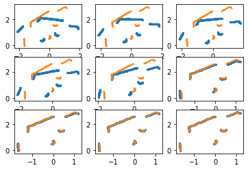
我们将每一次匹配之后的结果都画出来，可见ICP矫正匹配的速度还是非常快的

注意：

一，在实际应用ICP算法的过程中，我们需要求的是当前帧到上一帧的位姿变换

举个栗子：

一辆正在缓缓前进的小车，前方有一堵墙。假设小车向前移动了0.5m的距离

那么收集到的前一帧的点云会比较远，后一帧的点云会相对比较近，我们需要求的是距离近的点云到远的点云的位移

因此是我们需要求的是从当前点云到上一帧点云的位姿变换

ROS2 + GAZEBO 仿真代码实例

实例运行：

ros2 launch robot_description gazebo_lab_world.launch.py
ros2 run teleop_key_control teleop_key_control
ros2 run my_slam icp

二，迭代次数

theta = 3.1415926 / 3
t = np.array([0.01, 0.02])
R = np.array([[np.cos(theta), -np.sin(theta)], [np.sin(theta), np.cos(theta)]])
y_data_now = (R @ y_data_pre.T).T + t

def error(R):
    angle = np.arctan2(R[1, 0], R[0, 0]) 
    bias = np.array([R[0, 2], R[1, 2]])
    print("delta angle is: {}, delta t is {}".format((angle - theta) /3.1415926 * 180 , t - bias))

error(icpp(y_data_pre, y_data_now))

返回

iters: 33
delta angle is: -2.544443788574345e-14, delta t is [ 7.51135265e-16 -1.21777588e-15]

可以通过修改theta和t里面的值，大致都需要30多次的迭代。

但是旋转的角度不可以太大，例如旋转角度为90度的时候，就无力回天了

theta = 3.1415926 / 2
t = np.array([0.01, 0.02])

三，匹配点对的筛选

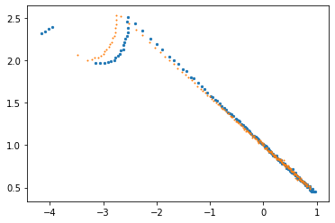
当机器人旋转的时候，会出现多个无法匹配的点，比如如下情况

因为在旋转的时候左上角的四个点，按照搜索最近的点无法获得匹配正确的情况，如果按照我们之前所介绍的ICP计算过程，其结果只能达到如下效果

因此在计算匹配点的时候，最近的点需要设立一个阈值，如最近点距离大于0.5就放弃这个点，不再进行匹配，下面对匹配函数进行修改

def find_correspend_point(y_data_pre, y_data_now):
    # 寻找对应点, 建立上一帧数据的KD树，循环下一帧的点
    # 寻找距离此点最近的在上一帧中的数据，保存到data_from_pre
    kdt = KDTree(y_data_now)
    data_from_now = []
    delete_idx = []
    for point_idx in range(y_data_pre.shape[0]):
        point = y_data_pre[point_idx:point_idx+1]
        dist, idx = kdt.query(point, k=1)
        if dist > 0.5:
            delete_idx.append(point_idx)
            continue
        data_from_now.append(y_data_now[idx.squeeze()])
    if delete_idx:
        delete_idx = np.array(delete_idx)
        y_data_pre = np.delete(y_data_pre, delete_idx, axis=0)

    return y_data_pre, np.array(data_from_now)

通过设定阈值，上述的数据为

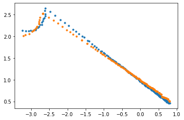
经过ICP迭代匹配，其结果是令人满意的

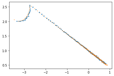
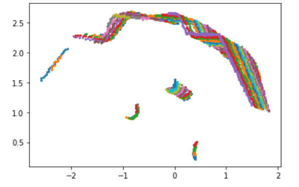
对于一次转弯的数据，应用上述的ICP方法，我们可以看见每一帧都对应匹配的还可以

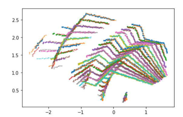
但是当我们把所有的匹配又根据当前的位姿返回到第一帧的时候，就可以看出还是差点意思

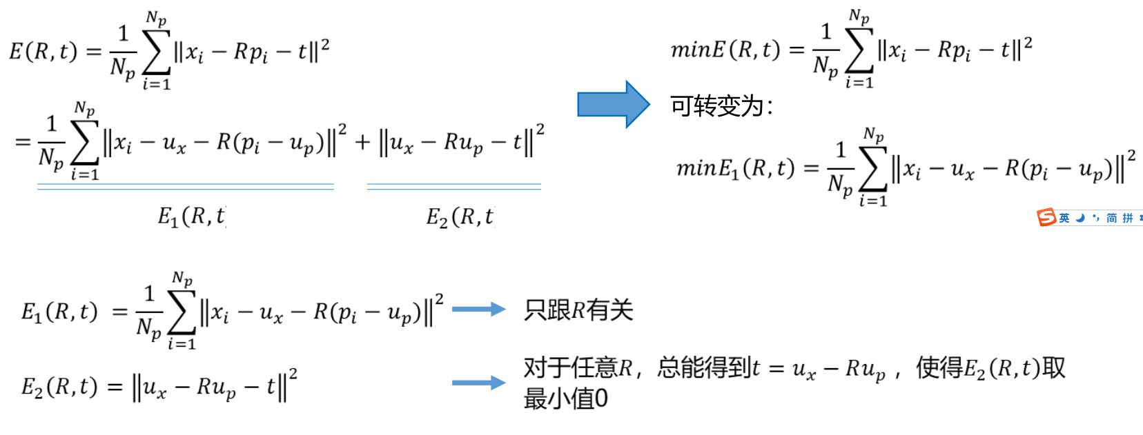
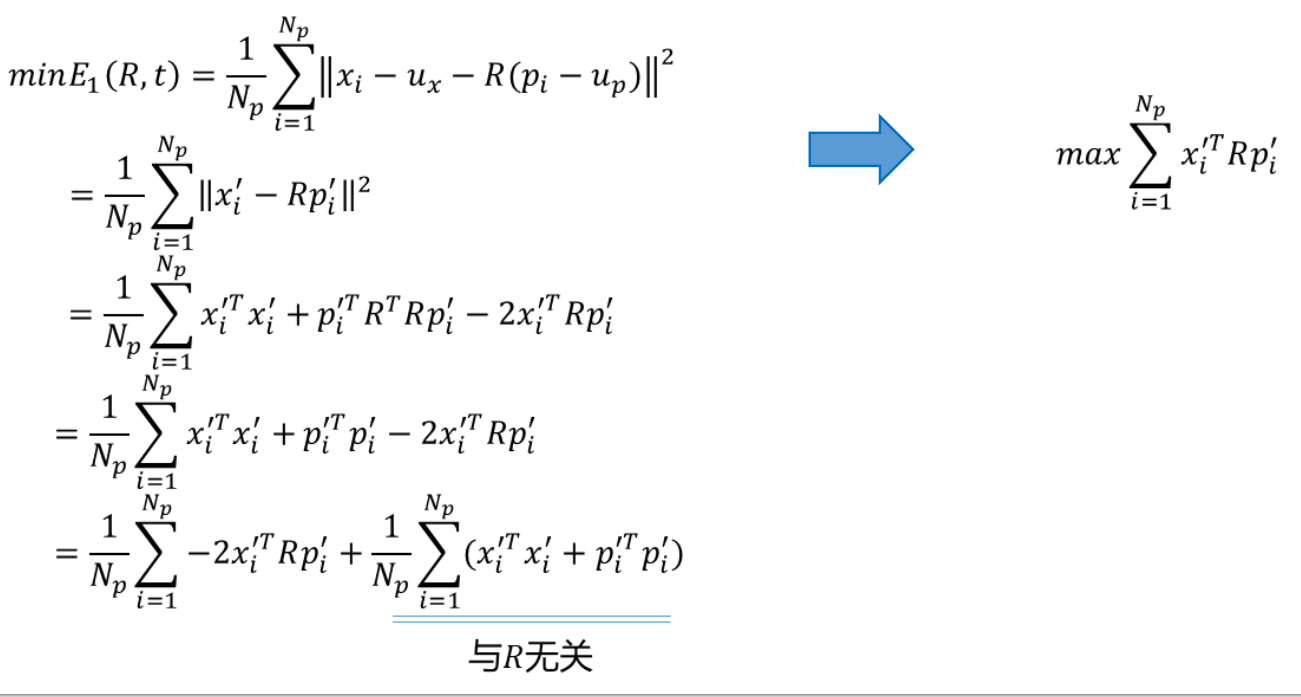
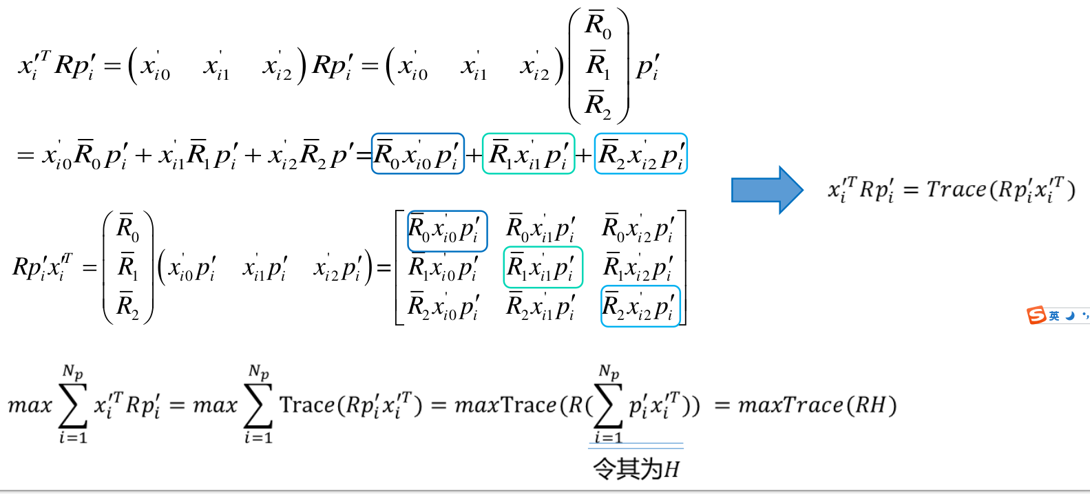
ICP 理论推导